BPM data
During stable operations in a storage ring/synchrotron, the beam is maintained on a closed orbit using feedback systems. The BPM data reflects this by showing a stable DC (average) position around zero (beam centroid) and stays within the noise range of the system. The noise is typically on the order of micrometers, and is caused by various environmental and machine-related errors.
When the beam is kicked using a fast kicker (\(\delta p_x\) and \(\delta p_y\)), the beam undergoes transverse, betatron oscillations. The beam is momentarily displaced from the orbit. The beam centroid naturally decays due to radiation damping and decoherence. During this process, the average position of the beam tends towards zero. Meanwhile the beam’s emittance increases until it reaches an equilibrium.
Below is an interactive animation of this process happening for one dimension in, say, an ideal storage ring. On the left is a gaussian beam with a kicked by \(\delta p = 0.2\) units. The working point was set to \(\nu_0 = 0.31\) and the tune spread was set to \(\sigma_{\nu} = 0.0025\). Each particle moves around the origin according to its own individual tune (in real life, this also changes with time, causing chaos). The tune spread (caused by many factors) is what causes this decoherence of the beam centroid in the animation. The beam centroid is plotted in red dots in both plots, and is what creates the turn-by-turn (TBT) data on the right.
(\(N_{particle}=5000, \beta=1, \alpha=0, \epsilon=0.005, N_{turn}=200\))
The BPM data can be approximated from the paper Decoherence Of Kicked Beams as a decaying sinusoid. Their final model incorporates two types of decoherence: decoherence from chromatic and nonlinear effects. We simplify their model a bit further to decrease the number of parameters that we have to work with:
\[x_{co}(N) = A\exp(-b N^2)\sin(2 \pi \nu N + \phi)\]Where \(x_{co}(N)\) is the closed-orbit position of the beam centroid as a function of turn number \(N\), \(A\) is the “position amplitude” of the kick, \(b\) is the decoherence factor, \(\nu\) is the tune and \(\phi\) is the phase offset. This approximation assumes no synchrotron radiation and other collective effects and only includes decoherence from chromatic effects. Therefore, a small angle approximation with respect to N was used. At RHIC, the synchrotron tune is much less than the betatron tunes, so only \(N = 200\) is usually used for measurements. A plot of the fit in orange using the equation above is shown below:
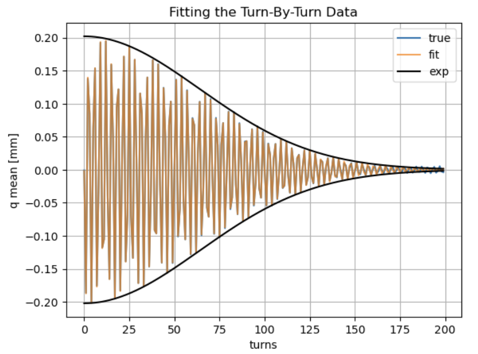
The black curves are plotted using the resulting parameters \(A, b\) on the exponential portion of \(x(n)\):
\[x(N) = A\exp(-b N^2)\]AC Dipoles were also used in RHIC in part to help with optics measurements. This was done by applying a sinusoidal (AC), oscillating magnetic field close to the working point, inducing coherent betatron oscillations into the beam. This allowed the BPM data to be approximated as just a sinusoidal function.
Realistically, aside from other causes of decoherence and tune shift, there are also BPM errors to take into account.
BPM Errors
Systematic errors from BPMs (physical errors of BPMs) come from a couple main sources: misalignment, tilt, gain/callibration, and coupling. Since these are systematic, they can be written in the following form:
\[\begin{pmatrix} \bar{x} \\ \bar{y} \end{pmatrix} = \frac{1}{\sqrt{1 - C^2}} \begin{pmatrix} \cos{\theta} && \sin{\theta} \\ -\sin{\theta} && \cos{\theta} \end{pmatrix} \begin{pmatrix} 1 && C \\ C && 1 \end{pmatrix} \begin{pmatrix} g_x && 0 \\ 0 && g_y \end{pmatrix} \begin{pmatrix} x \\ y \end{pmatrix}\]- \(x, y\): Data without BPM errors
- \(\bar{x}, \bar{y}\): Data with BPM errors
- \(g_x, g_y\): Gain/Callibration
- \(C\): Coupling
- \(\theta\): Roll
The remaining sources of errors usually stem from a multitude of causes such as vibrations and temperature. These errors are usualy random, and by the central limit theorem, they are usually taken to be gaussian. Many sources for RHIC deem random errors to be on the order of 5-30 \(\mu m\) depending where the BPM is around the ring.
Below is an interactive plot of the same BPM simulated data as before, but with a vertical axis as before (right column). The decoherence usually is very similar between bpms and axis, and the phase is usually random so those are set. However, the user is able to change the tune offset and amplitudes of the beams. They are able to play around with the various types of BPM errors to get a feel for how BPM error influence BPM data. The top plots show the BPM data without (black) and with (red) noise, and the bottom plots show the difference between the two curves.