This section talks explores a method to measuring the Beta Function involving Linear Least Squares (Linear Regression). We will first explore the linear least squares methods as well as short-comings and remedies. Then we will apply these to simulated RHIC BPM data.
Linear Least Squares
Linear Least Squares Methods minimize the distances between a linear equation and the points of a dataset:
\[Y = MX + B + \epsilon_y\]Where X and Y are points of the dataset retrieved from experiment/ simulation, and M and B are the parameters to fit the dataset. \(\epsilon_y\) is any errors that come from \(Y\). We call this regression method Ordinary Least Squares (OLS).
Ordinary Least Squares (OLS)
OLS can be a single or multi-variable method. For example, if Y depends on a single variable, \(X\) and \(Y\) are vectors and \(M, B\), and \(\epsilon_y\) are scalars. For the general case, \(X\) and \(Y\) will have the same shape that is \(m \times n \times N\), where \(m \times n\) is the number of vectors for OLS and \(N\) is the length of each vector. \(M, B\), and \(\epsilon_y\) subsequently has shape \(m \times n\) associated with each vector, i.e., every slope, y-intercept, and error is associated with every vector of \(X\).
Multivariate case:
For the \(i\)th data point where \(i \in N\):
\[\begin{pmatrix} Y^{11}_i && Y^{12}_i \\ Y^{21}_i && Y^{22}_i \end{pmatrix} = \begin{pmatrix} M^{11} && M^{12} \\ M^{21} && M^{22} \end{pmatrix} \cdot \begin{pmatrix} X^{11}_i && X^{12}_i \\ X^{21}_i && X^{22}_i \end{pmatrix} + \begin{pmatrix} B^{11} && B^{12} \\ B^{21} && B^{22} \end{pmatrix} + \begin{pmatrix} \epsilon^{11}_y && \epsilon^{12}_y \\ \epsilon^{21}_y && \epsilon^{22}_y \end{pmatrix}\]Where:
\[Y^{mn}_i = \begin{pmatrix} Y^{mn}_1 && Y^{mn}_2 && ... && Y^{mn}_N \end{pmatrix}\] \[X^{mn}_i = \begin{pmatrix} X^{mn}_1 && X^{mn}_2 && ... && X^{mn}_N \end{pmatrix}\]And each element in \(M\) is multiplied element-wise to \(X_i\). This is such that when you keep track of one element, it looks like the single-variable case.
For the least squares equation, the mean of the dataset is a standard guess for \(B\) and is subtracted out. The solution to the OLS regression in matrix form is therefore:
\[M = (X^TX)^{-1}X^TY\]There are certain assumptions when using OLS:
- Linearity: \(Y\) can be made from a linear combination of all independent variables \(X\).
- Independence of errors: All errors are independent from each other and of the independent variables themselves.
- No Co-linearity: All independent variables are independent from each other.
- Homoscedasticity: Assumes the variance between variables in \(Y\) (\(\epsilon_y^2\)) remains constant for all values of the independent variables \(X\)
- Errors-in-variables: The independent variables \(X\) contain no errors, or that those errors that are much smaller than the range of \(X\) values that can be attained.
When the homoscedasticity assumption is violated, one can use weighted least squares for an estimate for \(M\). If homoscedasticity and independence of errors are both violated, generalized least squares can be utilized.
However, the focus of this article is on when the errors in variables assumption is violated. When this happens, one can use a method called total least squares to get an estimate for \(M\). Before doing so, we should see what happens when it is violated to see what to look out for.
If there is error in the X variable (\(\epsilon_x\)), the OLS equation then looks like:
\[Y = M(X + \epsilon_x) + B + \epsilon_y\]Plotting \(\epsilon_x\) vs estimates of the slope using OLS yields:
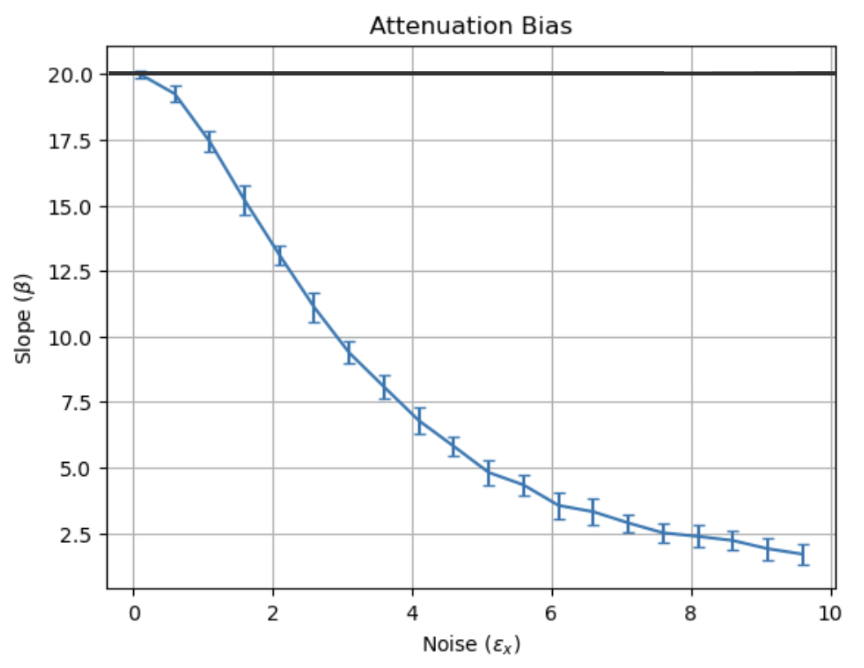
This is called attenuation bias, and the estimate of the slope gets worse as \(\epsilon_x\) increases, rendering OLS untrustworthy for larger noise values. Mathematically, the relationship between the measured slope \(\hat{\beta}\) (\(\beta\) is used as slope in statistics, \(M\) is also still slope) and the real slope \(\beta\) is given by:
\[\hat{\beta} = \frac{\beta \sigma_x^2}{\sigma_x^2 + \epsilon_x^2}\]Where \(\sigma_x\) is the intended range of \(x\) values taken on. OLS only then works if \(\epsilon_x << \sigma_x\). The error bars in fig. 1 also seems constant as the error in x changes.
Total Least Squares (TLS)
One way to address the violation of errors in variables is to use a method known as total least squares. This method takes into account the noise in independent variables by taking advantage of singular value decomposition (SVD). The idea of SVD is to identify the least amount of components of the dataset that will most reconstruct it. Consequently
TLS attempts to minimize the error in both \(\boldsymbol{X}\) and \(\boldsymbol{Y}\), namely \(\boldsymbol{E}\) and \(\boldsymbol{F}\):
\[\begin{aligned} (\hat{\boldsymbol{M}}_j,\hat{\boldsymbol{E}},\hat{\boldsymbol{F}}) &= \text{argmin}_{\boldsymbol{M}_j,\boldsymbol{E},\boldsymbol{F}} \left\| \begin{bmatrix} \boldsymbol{E} & \boldsymbol{F} \end{bmatrix} \right\|_F, \\ \text{subject to}\quad \boldsymbol{Y} + \boldsymbol{F} &= \boldsymbol{M}_j \bigl(\boldsymbol{X} + \boldsymbol{E}\bigr). \end{aligned}\]Where \(\|\cdot\|_F\) denotes the Frobenius norm. An (SVD) of the concatenation of \(\boldsymbol{X}\) and \(\boldsymbol{Y}\) is taken:
\[\begin{equation} \begin{bmatrix} \boldsymbol{X} & \boldsymbol{Y} \end{bmatrix} = \begin{bmatrix} \boldsymbol{U}_X & \boldsymbol{U}_Y \end{bmatrix} \begin{bmatrix} \boldsymbol{\Sigma}_x & 0 \\ 0 & \boldsymbol{\Sigma}_Y \end{bmatrix} \begin{bmatrix} \boldsymbol{V}_{XX} & \boldsymbol{V}_{XY} \\ \boldsymbol{V}_{YX} & \boldsymbol{V}_{YY} \end{bmatrix}^* \end{equation}\]and the solution for \(\boldsymbol{M}_j\) is given by:
\[\begin{equation} \boldsymbol{M}_j = -\boldsymbol{V}_{XY}\boldsymbol{V}_{YY}^{-1} \end{equation}\]A detailed derivation can be found here:
Golub, Gene H., and Charles F. Van Loan. “An analysis of the total least squares problem.” SIAM journal on numerical analysis 17.6 (1980): 883-893.
Generalized Total Least Squares (GTLS)
OLS slope: —
TLS slope: —
Observations
- High \(\epsilon_x\), low \(\epsilon_y\), high \(\|m\|\): TLS gives a better estimate for increasing slopes compared to OLS
- increasing or decreasing \(\epsilon_x, \epsilon_y\): TLS still yields better estimates than OLS for high \(\|m\|\)
- High \(\epsilon_x\), low \(\epsilon_y\), low \(\|m\|\): TLS and OLS give similar solid estimates for the slope
- increasing \(\epsilon_y >> \epsilon_x\): OLS yields better estimates than TLS
- The variation in TLS depends linearly \(\epsilon_x\); for high \(\epsilon_x\), there is high variation in TLS.
Least Squares for BPM Measurements
Might be biased for RHIC collider?